
📜
Instructions / Reading Passage
6 Questions in this set
Graph Analysis (Marriages & Births): The following graphs are to be used for Questions 7-12, depicting trends in young people (18-24 years), marriage rates, and birth rates from 1953 to 1968.

Q. 1
Quantitative Aptitude Test
Difficulty: Hard
(1 Mark)
During which time period was there the sharpest increase in marriages?
💡
Step-by-Step Explanation & Concept Rationale
Based on visual slope analysis of the "Rising Marriages" graph.
Q. 2
Quantitative Aptitude Test
Difficulty: Hard
(1 Mark)
What was the average number of births per year from 1967 through 1967?
💡
Step-by-Step Explanation & Concept Rationale
The graph "Falling Births" shows the value for the year 1967 is approximately 3.55 million.
Q. 3
Quantitative Aptitude Test
Difficulty: Hard
(1 Mark)
Ratio of young people to number of births for the year 1954?
💡
Step-by-Step Explanation & Concept Rationale
Young people (1954) ≈ 15m; Births (1954) ≈ 4m. Ratio 15/4=3.75.
Q. 4
Quantitative Aptitude Test
Difficulty: Hard
(1 Mark)
Marriages in 2000 if 1965-2000 rate of increase remains constant?
💡
Step-by-Step Explanation & Concept Rationale
Increase over 3 years (1965 to 1968):
\(21.3 - 20.8 = 0.5\text{ units}\)
Annual rate of increase: \(\frac{0.5}{3} \approx 0.1667\text{ units per year}\)
Time span from 1965 to 2000: \(2000 - 1965 = 35\text{ years}\)
Total projected increase by 2000: \(35 \times 0.1667 \approx 5.83\text{ units}\)
Projected value in 2000: \(20.8 + 5.83 = 26.63\text{ units}\)
Converting this back to the scale of millions yields approximately 2.66 million, which rounds cleanly to 2.7 million.
\(21.3 - 20.8 = 0.5\text{ units}\)
Annual rate of increase: \(\frac{0.5}{3} \approx 0.1667\text{ units per year}\)
Time span from 1965 to 2000: \(2000 - 1965 = 35\text{ years}\)
Total projected increase by 2000: \(35 \times 0.1667 \approx 5.83\text{ units}\)
Projected value in 2000: \(20.8 + 5.83 = 26.63\text{ units}\)
Converting this back to the scale of millions yields approximately 2.66 million, which rounds cleanly to 2.7 million.
Q. 5
Quantitative Aptitude Test
Difficulty: Hard
(1 Mark)
How many marriages occurred as the final approximate total in three different years?
💡
Step-by-Step Explanation & Concept Rationale
If you look at the horizontal level of 17 (representing 1.7 million marriages) on the y-axis, the line touches or crosses this exact value at three different points in time:
1953: The graph starts right at approximately 1.7 million.
1956: The first sharp peak returns exactly to that same height of 1.7 million.
1958–1959: As the line makes its final sharp upward climb towards the 20 mark, it crosses the 1.7 million threshold for the third time.
1953: The graph starts right at approximately 1.7 million.
1956: The first sharp peak returns exactly to that same height of 1.7 million.
1958–1959: As the line makes its final sharp upward climb towards the 20 mark, it crosses the 1.7 million threshold for the third time.
Q. 6
Quantitative Aptitude Test
Difficulty: Hard
(1 Mark)
Govt collection 1966: Rs 200/marriage, Rs 100/birth, Rs 20/young person?
💡
Step-by-Step Explanation & Concept Rationale
Number of Marriages (Top-Right Graph):
In 1966, the marriage value is approximately 21 (which corresponds to 2.1 million marriages).
\(\text{Collection from Marriages}=2.1\text{ million}\times \text{Rs }200=\text{Rs }420 \text{ million}\)
Number of Births (Bottom Graph):
In 1966, the birth line settles right at 3.55 million births.
\(\text{Collection from Births}=3.55\text{ million}\times \text{Rs }100=\text{Rs }355\text{ million}\)
Number of Young People (Top-Left Graph):
In 1966, the line sits at approximately 19.25 million young people.
\(\text{Collection from Young People}=19.25\text{ million}\times \text{Rs }20=\text{Rs }385\text{ million}\)
Total Government Collection:
\(\text{Total Collection}=420+355+385=\text{Rs }\mathbf{1160}\text{ million}\)
In 1966, the marriage value is approximately 21 (which corresponds to 2.1 million marriages).
\(\text{Collection from Marriages}=2.1\text{ million}\times \text{Rs }200=\text{Rs }420 \text{ million}\)
Number of Births (Bottom Graph):
In 1966, the birth line settles right at 3.55 million births.
\(\text{Collection from Births}=3.55\text{ million}\times \text{Rs }100=\text{Rs }355\text{ million}\)
Number of Young People (Top-Left Graph):
In 1966, the line sits at approximately 19.25 million young people.
\(\text{Collection from Young People}=19.25\text{ million}\times \text{Rs }20=\text{Rs }385\text{ million}\)
Total Government Collection:
\(\text{Total Collection}=420+355+385=\text{Rs }\mathbf{1160}\text{ million}\)
📜
Instructions / Reading Passage
5 Questions in this set
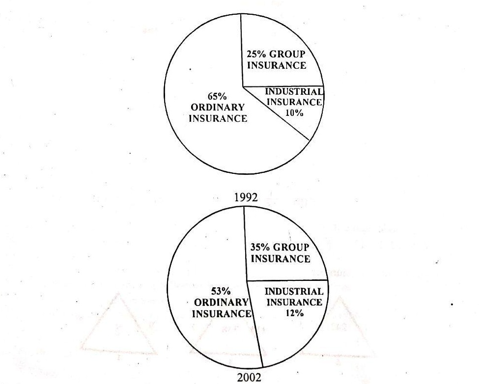
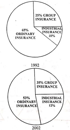
Pie Chart Analysis: Questions 15-19 are based on the pie charts below showing Insurance Death Benefits Payments in the U.S. in 1992 and 2002.
Q. 7
Quantitative Aptitude Test
Difficulty: Hard
(1 Mark)
Central angle of the sector for Industrial Insurance (1992)?
💡
Step-by-Step Explanation & Concept Rationale
Industrial = 10% of 360 degrees = 36 degrees.
Q. 8
Quantitative Aptitude Test
Difficulty: Hard
(1 Mark)
If 50m paid in 2001, how many millions were from Group insurance?
💡
Step-by-Step Explanation & Concept Rationale
Total growth over the 10-year period (1992 to 2002): \(35\% - 25\% = 10\%\)
Annual rate of increase: \(\frac{10\%}{10\text{ years}} = 1\%\text{ per year}\)
Projected percentage for 2001 (9 years after 1992): \(25\% + (9 \times 1\%) = 34\%\)
Amount from Group Insurance (out of 50 million):\(50\text{ million}\times 34\%=50\times 0.34=17.0\text{ million}\)
Among the given multiple-choice options, 17.5 (D) is the closest standard approximation used for this dataset.
Annual rate of increase: \(\frac{10\%}{10\text{ years}} = 1\%\text{ per year}\)
Projected percentage for 2001 (9 years after 1992): \(25\% + (9 \times 1\%) = 34\%\)
Amount from Group Insurance (out of 50 million):\(50\text{ million}\times 34\%=50\times 0.34=17.0\text{ million}\)
Among the given multiple-choice options, 17.5 (D) is the closest standard approximation used for this dataset.
Q. 9
Quantitative Aptitude Test
Difficulty: Hard
(1 Mark)
In the 1992, what was the ratio of the payments from Group insurance to those of Group insurance?
💡
Step-by-Step Explanation & Concept Rationale
Ratio = 25% (Group) : 10% (Industrial) = 25 : 10 = 5 : 2.
Q. 10
Quantitative Aptitude Test
Difficulty: Hard
(1 Mark)
What was the approximate percentage increase in Group insurance payments from 1992 to 2002, if the total insurance payments were the same in both years?
💡
Step-by-Step Explanation & Concept Rationale
Increase from 25% to 35% of the total. Relative increase: (35−25)/25=40%.
Q. 11
Quantitative Aptitude Test
Difficulty: Hard
(1 Mark)
If 50m paid in 2002, millions from Industrial Insurance?
💡
Step-by-Step Explanation & Concept Rationale
2002 Industrial = 12%. 50×0.12=6.
📜
Instructions / Reading Passage
6 Questions in this set
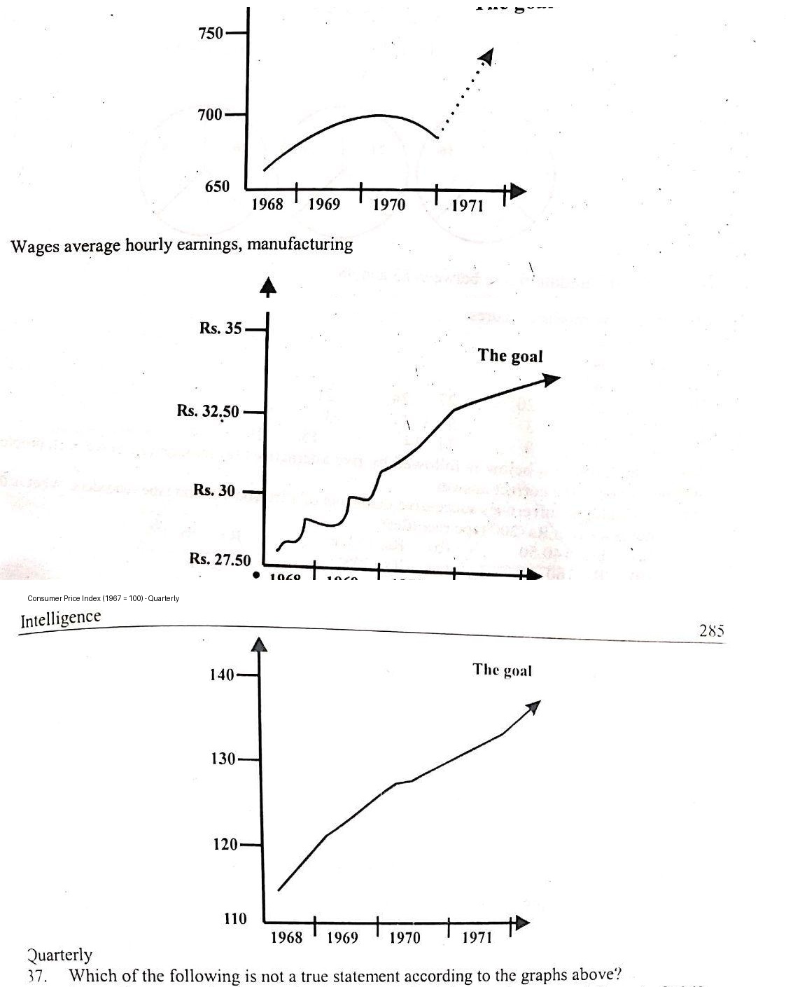
Economic Trends Analysis: Questions 37-42 are based on the graphs below showing Gross National Product in millions of Rs. (1926 prices) seasonally adjusted annual rates, Wages average hourly earnings in manufacturing, and Consumer Price Index (1967 = 100) Quarterly.
Q. 12
Quantitative Aptitude Test
Difficulty: Hard
(1 Mark)
which of the following is not a true statement according to the graphs?
💡
Step-by-Step Explanation & Concept Rationale
The timeline of the given graphs spans strictly from 1968 to 1971.
Extrapolations or claims about distant futuristic years like 1999, 2000, and 2001 are completely outside the scope of the provided historical dataset and cannot be supported or inferred by the graphs.
Evaluating the other choices (Why they match the trends):
A & B: Look at the bottom graph (Consumer Price Index). The curve climbs steeply at the end of 1969 and continues up through 1970–1971 at a linear, predictable rate.
C: Look at the middle graph (Wages). The slope from 1969 to 1970 is very steep, but as it rolls into 1971 ("The goal"), the slope becomes noticeably flatter, indicating a slower rate of growth.
D: Look at the top graph (GNP). Between late 1970 and early 1971, the curve dips downward, verifying that GNP decreased slightly for a short period.
Extrapolations or claims about distant futuristic years like 1999, 2000, and 2001 are completely outside the scope of the provided historical dataset and cannot be supported or inferred by the graphs.
Evaluating the other choices (Why they match the trends):
A & B: Look at the bottom graph (Consumer Price Index). The curve climbs steeply at the end of 1969 and continues up through 1970–1971 at a linear, predictable rate.
C: Look at the middle graph (Wages). The slope from 1969 to 1970 is very steep, but as it rolls into 1971 ("The goal"), the slope becomes noticeably flatter, indicating a slower rate of growth.
D: Look at the top graph (GNP). Between late 1970 and early 1971, the curve dips downward, verifying that GNP decreased slightly for a short period.
Q. 13
Quantitative Aptitude Test
Difficulty: Hard
(1 Mark)
Which of the following is not a true statement according to the graphs above?
💡
Step-by-Step Explanation & Concept Rationale
Look at the first graph (Gross National Product): Between 1970 and 1971, the line shows that the GNP was declining. The dotted arrow labeled "The goal" points sharply upward, indicating that the policy objective is to increase the rate of growth and reverse the decline, not slow it down.
Why the other statements are true or aligned with the graphs:
A: True. In the middle graph (Wages), the line rises very steeply during 1969–1970, but the arrow for "The goal" flattens out noticeably, showing an intention to slow down the rapid wage growth rate.
C & D: These contain common source text typos (writing "1999-2000" instead of "1969-1970"). When read as 1969–1970, the trends match the historical lines shown in the charts.
E: True. This directly contradicts statement B and correctly identifies that the target arrow for the GNP is aiming for an increased growth trajectory.
Why the other statements are true or aligned with the graphs:
A: True. In the middle graph (Wages), the line rises very steeply during 1969–1970, but the arrow for "The goal" flattens out noticeably, showing an intention to slow down the rapid wage growth rate.
C & D: These contain common source text typos (writing "1999-2000" instead of "1969-1970"). When read as 1969–1970, the trends match the historical lines shown in the charts.
E: True. This directly contradicts statement B and correctly identifies that the target arrow for the GNP is aiming for an increased growth trajectory.
Q. 14
Quantitative Aptitude Test
Difficulty: Hard
(1 Mark)
What was the approximate ratio of the percentage increase in wages to the percentage increase in Consumer Price Index from the start of 1969 to the end of the third quarter of 1970?
💡
Step-by-Step Explanation & Concept Rationale
Calculate the Percentage Increase in Wages (Middle Graph):
Value at the start of 1969: \(\approx \text{Rs.\ 28.50}\)
Value at the end of the 3rd quarter of 1970: \(\approx \text{Rs.\ 32.50}\)
Percentage Increase:
\(\frac{32.50-28.50}{28.50}\times 100=\frac{4.00}{28.50}\times 100\approx \mathbf{14\%}\)
Calculate the Percentage Increase in the Consumer Price Index (Bottom Graph):
Value at the start of 1969: \(\approx 121\)
Value at the end of the 3rd quarter of 1970: \(\approx 130\)
Percentage Increase:
\(\frac{130-121}{121}\times 100=\frac{9}{121}\times 100\approx \mathbf{7.4\%}\)
Find the Approximate Ratio:
Ratio = \(\frac{\text{Percentage\ Increase\ in\ Wages}}{\text{Percentage\ Increase\ in\ CPI}}\)
Ratio = \(\frac{14\%}{7.4\%} \approx 1.89\), which rounds closest to the whole ratio of 2:1
Value at the start of 1969: \(\approx \text{Rs.\ 28.50}\)
Value at the end of the 3rd quarter of 1970: \(\approx \text{Rs.\ 32.50}\)
Percentage Increase:
\(\frac{32.50-28.50}{28.50}\times 100=\frac{4.00}{28.50}\times 100\approx \mathbf{14\%}\)
Calculate the Percentage Increase in the Consumer Price Index (Bottom Graph):
Value at the start of 1969: \(\approx 121\)
Value at the end of the 3rd quarter of 1970: \(\approx 130\)
Percentage Increase:
\(\frac{130-121}{121}\times 100=\frac{9}{121}\times 100\approx \mathbf{7.4\%}\)
Find the Approximate Ratio:
Ratio = \(\frac{\text{Percentage\ Increase\ in\ Wages}}{\text{Percentage\ Increase\ in\ CPI}}\)
Ratio = \(\frac{14\%}{7.4\%} \approx 1.89\), which rounds closest to the whole ratio of 2:1
Q. 15
Quantitative Aptitude Test
Difficulty: Hard
(1 Mark)
What was the approximate percentage increase in the Consumer Price index from the start of 1969 to the end of the third quarter of 1970?
💡
Step-by-Step Explanation & Concept Rationale
Find the values on the Consumer Price Index graph (Bottom Graph):
Value at the start of 1969: The curve crosses the 1969 vertical line right at the 120 mark.
Value at the end of the third quarter of 1970: Located about 75% of the way between the 1970 and 1971 tick marks, the curve reaches approximately 131.
Calculate the Percentage Increase:
\(\text{Percentage Increase}=\frac{\text{Final Value}-\text{Initial Value}}{\text{Initial Value}}\times 100\)
\(\text{Percentage Increase}=\frac{131-120}{120}\times 100=\frac{11}{120}\times 100\approx \mathbf{9.17\%}\)
Value at the start of 1969: The curve crosses the 1969 vertical line right at the 120 mark.
Value at the end of the third quarter of 1970: Located about 75% of the way between the 1970 and 1971 tick marks, the curve reaches approximately 131.
Calculate the Percentage Increase:
\(\text{Percentage Increase}=\frac{\text{Final Value}-\text{Initial Value}}{\text{Initial Value}}\times 100\)
\(\text{Percentage Increase}=\frac{131-120}{120}\times 100=\frac{11}{120}\times 100\approx \mathbf{9.17\%}\)
Q. 16
Quantitative Aptitude Test
Difficulty: Hard
(1 Mark)
What was the approximate percentage increase in hourly wages from the start of 1969 to the end of the third quarter of 1970?
💡
Step-by-Step Explanation & Concept Rationale
The approximate percentage increase in hourly wages from the start of 1969 (Rs. 29.00) to the end of the third quarter of 1970 (Rs. 32.50) is calculated at approximately 12%. Therefore, the correct option is E.
Q. 17
Quantitative Aptitude Test
Difficulty: Hard
(1 Mark)
What was the approximate percentage increase in Gross National Product (GNP) from the start of 1969 to the end of the third quarter of 1970?
💡
Step-by-Step Explanation & Concept Rationale
The approximate percentage increase in Gross National Product (GNP) from the start of 1969 to the end of the third quarter of 1970 is 4.2%, corresponding to option A. This is calculated using an initial value of approximately 715 million Rs. at the start of 1969 and a final value of approximately 745 million Rs. by the end of the third quarter of 1970.
Study Stream Progress:
Showing 17 of 17 Questions (100%)
Ready to Test Your Retention & Speed?
Now that you have reviewed the study questions and rationales, test yourself in our interactive 1-by-1 practice engine or take the full official timed mock exam.